Previous part

• Arnoldi orthogonalization of Krylov subspaces
• Lanczos for the symmetric case
• Energy functional and conjugate gradient method
• Convergence analysis
• Non-symmetric case: idea of GMRES

Now we will cover the following topics

• More iterative methods: MINRES, BiCG and BiCGStab
• The concept of preconditioners

What methods to use

• If a matrix is symmetric (Hermitian) positive definite, use CG method.
• If a matrix is symmetric but indefinite, we can use MINRES method (GMRES applied to a symmetric system)
• If a matrix is non-symmetric and not very big, use GMRES
• If a matrix is non-symmetric and we can store limited amount of vectors, use either: GMRES with restarts, or BiCGStab (the latter of the product with A^{\top} is also available).

More detailed flowchart from this book

MINRES

The MINRES method is GMRES applied to a symmetric system.

• We search the solution in the subspace spanned by columns of Q_j

x_j = x_0 + Q_j c_j

• We minimize the residual norm

\Vert Ax_j - f\Vert_2 = \Vert Ax_0 + AQ_j c_j - f\Vert_2 = \Vert A Q_j c_j - r_0 \Vert_2 = \Vert Q_j H_j c_j + h_{j, j-1} q_j c_j - r_0 \Vert_2 = \Vert Q_{j+1} \widetilde{H}_{j+1} c_j - r_0 \Vert_2 \rightarrow \min_{c_j}

which is equivalent to a linear least squares with an almost tridiagonal matrix

\Vert \widetilde{H}_{j+1} c_{j} - \gamma e_0 \Vert_2 \rightarrow \min_{c_{j}}.

• In a similar fashion, we can derive short-term recurrences.

• A careful implementation of MINRES requires at most 5 vectors to be stored.

Difference between MINRES and CG

• MINRES minimizes \Vert Ax_k - f \Vert_2 over the Krylov subspace
• CG minimize (Ax, x) - 2(f, x) over the Krylov subspace
• MINRES works for indefinite (i.e., non-positive definite) problems.

CG stores less vectors (3 instead of 5).

Now, let us talk about non-symmetric systems.

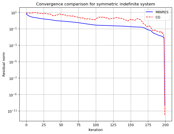
import scipy.sparse.linalg
import matplotlib.pyplot as plt
import numpy as np
import scipy as sp

# Create a symmetric indefinite matrix
n = 200
diag = np.ones(n)
# Create a discretized 1D Helmholtz operator: -d^2/dx^2 - k^2
h = 1.0/n  # Grid spacing
k = 0     # Wave number

# Create diagonals for tridiagonal matrix
main_diag = -2.00/h**2 + k**2  # Main diagonal: -2/h^2 + k^2 
off_diag = 1.0/h**2           # Off diagonals: 1/h^2

# Create arrays for the three diagonals
main = np.ones(n) * main_diag
upper = np.ones(n) * off_diag  
lower = np.ones(n) * off_diag

# Construct tridiagonal matrix using sparse diagonals
# The error occurs because spdiags expects diagonals to be provided in a 2D array
# where each row represents a diagonal. Let's stack them correctly:
A = sp.sparse.spdiags([lower, main, upper], [-1, 0, 1], n, n, format='csr')
# Random right-hand side
np.random.seed(42)
b = np.random.randn(n)

# Lists to store residual norms
res_minres = []
res_cg = []

def callback_minres(xk):
    res_minres.append(np.linalg.norm(b - A @ xk))
    
def callback_cg(xk):
    res_cg.append(np.linalg.norm(b - A @ xk))

# Solve with MINRES
x_minres = scipy.sparse.linalg.minres(A, b, callback=callback_minres, maxiter=500, rtol=1e-10)

# Try to solve with CG (may not converge due to indefiniteness)
try:
    x_cg = scipy.sparse.linalg.cg(A, b, callback=callback_cg, maxiter=500, rtol=1e-10)
except:
    print("CG failed to converge as expected for indefinite system")

# Plot convergence
plt.figure(figsize=(8, 6))
plt.semilogy(res_minres, 'b-', label='MINRES')
if len(res_cg) > 0:
    plt.semilogy(res_cg, 'r--', label='CG')
plt.xlabel('Iteration')
plt.ylabel('Residual norm')
plt.title('Convergence comparison for symmetric indefinite system')
plt.legend()
plt.grid(True)
np.max(np.linalg.eigvals(A.todense()))

np.float64(-9.771444747833783)

Non-symmetric systems

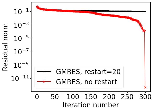
• The main disadvantage of GMRES: we have to store all the vectors, so the memory cost grows with each step.

• We can do restarts (i.e. get a new residual and a new Krylov subspace): we find some approximate solution x and now solve the linear system for the correction:

A(x + e) = f, \quad Ae = f - Ax,

and generate the new Krylov subspace from the residual vector. This spoils the convergence, as we will see from the demo.

import scipy.sparse.linalg
%matplotlib inline
import matplotlib.pyplot as plt
plt.rc("text", usetex=False)
import numpy as np
import scipy as sp

n = 300
ex = np.ones(n);
A = -sp.sparse.spdiags(np.vstack((ex,  -(2 + 1./n)*ex, (1 + 1./n) * ex)), [-1, 0, 1], n, n, 'csr'); 
rhs = np.random.randn(n)

res_gmres_rst = []
res_gmres = []
def gmres_rst_cl(r):
    res_gmres_rst.append(np.linalg.norm(r))
    
def gmres_rst(r):
    res_gmres.append(np.linalg.norm(r))

sol = scipy.sparse.linalg.gmres(A, rhs, restart=20, callback=gmres_rst_cl)
sol = scipy.sparse.linalg.gmres(A, rhs, restart=n, callback=gmres_rst)

lim = 300
plt.semilogy(res_gmres_rst[:lim], marker='.',color='k', label='GMRES, restart=20')
plt.semilogy(res_gmres[:lim], marker='x',color='r', label='GMRES, no restart')
plt.xlabel('Iteration number', fontsize=20)
plt.ylabel('Residual norm', fontsize=20)
plt.xticks(fontsize=20)
plt.yticks(fontsize=20)
plt.legend(fontsize=20)

How to avoid such spoiling of convergence?

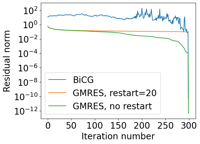
• BiConjugate Gradient method (named BiCG, proposed by Fletcher, original paper) avoids that using “short recurrences” like in the CG method.

Idea of biconjugate gradient

Idea of BiCG method is to use the normal equations:

A^* A x = A^* f,

and apply the CG method to it.

• The condition number has squared, thus we need stabilization.

• The stabilization idea proposed by Van der Vorst et al. improves the stability (later in the lecture)

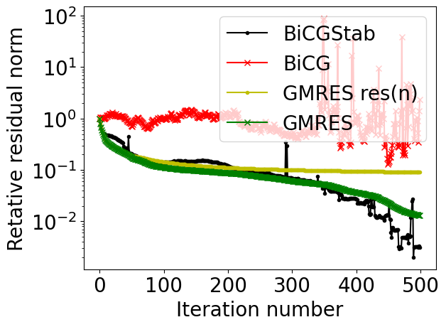
Let us do some demo for a simple non-symmetric matrix to demonstrate instability of BiCG method.

res_all_bicg = []
def bicg_cl(x):
    res_all_bicg.append(np.linalg.norm(A.dot(x) - rhs))
    
sol = scipy.sparse.linalg.bicg(A, rhs, x0=np.zeros(n), callback=bicg_cl)
plt.semilogy(res_all_bicg, label='BiCG')
plt.semilogy(res_gmres_rst[:n], label='GMRES, restart=20')
plt.semilogy(res_gmres, label='GMRES, no restart')
plt.xlabel('Iteration number', fontsize=20)
plt.ylabel('Residual norm', fontsize=20)
plt.xticks(fontsize=20)
plt.yticks(fontsize=20)
plt.legend(fontsize=20)

BiConjugate Gradients

There are two options:

1. Use \mathcal{K}(A^* A, A^* f) to generate the subspace. That leads to square of condition number
2. Instead, use two Krylov subspaces \mathcal{K}(A) and \mathcal{K}(A^*) to generate two basises that are biorthogonal (so-called biorthogonal Lanczos).

The goal is to compute the Petrov-Galerkin projection

W^* A V \widehat{x} = W^* f

with columns W from the Krylov subspace of A^*, V from A (cf. with CG case).

That may lead to instabilities if we try to recompute the solutions in the efficient way. It is related to the pivoting (which we did not use in CG), and it is not naturally implemented here.

Notes about BiCG

A practical implementation of BiCG uses two-sided Lanczos process: generating Krylov subspace for A and A^{\top}

In partucular

1. \alpha_j = \frac{(r_j, \hat{r}_j)}{(Ap_j, \hat{p}_j)}
2. $x_{j+1} = x_j + _j p_j $
3. r_{j+1} = r_j - \alpha_j Ap_j
4. \hat{r}_{j+1} = \hat{r}_j - \alpha_j A^{\top}\hat{p}_j
5. \beta_j = \frac{(r_{j+1}, \hat{r}_{j+1})}{(r_j, \hat{r}_j)}
6. p_{j+1} = r_{j+1} + \beta_j p_j
7. \hat{p}_{j+1} = \hat{r}_{j+1} - \beta_j \hat{p}_j

Now we move to the stable version of the BiCG method

BiCGStab

• BiCGStab is frequently used, and represent a stabilized version of BiCG. It has faster and smoother convergence than original BiCG method.

• The formulas can be found, for example, here

• It is a combination of BiCG step followed by GMRES(1) step in order to smooth the convergence.

• For more details, please consult the book “Iterative Krylov Methods for Large Linear Systems” by H. Van-der Vorst.

A short demo to compare “Stabilized” vs “Non-stabilized” versions.

import scipy.sparse.linalg
%matplotlib inline
import matplotlib.pyplot as plt
import numpy as np
import scipy as sp

n = 600

ex = np.ones(n);
A = -sp.sparse.spdiags(np.vstack((ex,  -(2 + 1./n)*ex, (1 + 1./n) * ex)), [-1, 0, 1], n, n, 'csr') 
rhs = np.random.randn(n)

# ee = sp.sparse.eye(n)
# A = -sp.sparse.spdiags(np.vstack((ex,  -(2 + 1./n)*ex, (1 + 1./n) * ex)), [-1, 0, 1], n, n, 'csr')
# A = sp.sparse.kron(A, ee) + sp.sparse.kron(ee, A)
# rhs = np.ones(n * n)

print("Dimension of the linear system = {}".format(A.shape[0]))

res_all_bicg = []
res_all_bicgstab = []
def bicg_cl(x):
    res_all_bicg.append(np.linalg.norm(A.dot(x) - rhs))

def bicgstab_cl(x):
    res_all_bicgstab.append(np.linalg.norm(A.dot(x) - rhs))

res_gmres_rst = []
res_gmres = []
def gmres_rst_cl(r):
    res_gmres_rst.append(np.linalg.norm(r))
    
def gmres_rst(r):
    res_gmres.append(np.linalg.norm(r))

sol2 = scipy.sparse.linalg.gmres(A, rhs, restart=20, callback=gmres_rst_cl)
sol2 = scipy.sparse.linalg.gmres(A, rhs, restart=n, callback=gmres_rst)

    
sol2 = scipy.sparse.linalg.bicg(A, rhs, x0=np.zeros(A.shape[0]), callback=bicg_cl)
sol2 = scipy.sparse.linalg.bicgstab(A, rhs, x0=np.zeros(A.shape[0]), callback=bicgstab_cl)
res_all_bicg = np.array(res_all_bicg)/res_all_bicg[0]
res_all_bicgstab = np.array(res_all_bicgstab)/res_all_bicgstab[0]
res_gmres_rst = np.array(res_gmres_rst)/res_gmres_rst[0]
res_gmres = np.array(res_gmres)/res_gmres[0]

lim = 500
plt.semilogy(res_all_bicgstab[:lim], marker='.',color='k', label='BiCGStab')
plt.semilogy(res_all_bicg[:lim], marker='x',color='r', label='BiCG')
plt.semilogy(res_gmres_rst[:lim], marker='.',color='y', label='GMRES res(n)')
plt.semilogy(res_gmres[:lim], marker='x',color='g', label='GMRES')

plt.xlabel('Iteration number', fontsize=20)
plt.ylabel('Retative residual norm', fontsize=20)
plt.legend(loc='best', fontsize=20)
plt.xticks(fontsize=20)
_ = plt.yticks(fontsize=20)

Dimension of the linear system = 600

“Nonlinear GMRES” or Anderson acceleration

We can apply the GMRES-like idea to speed up the convergence of a given fixed-point iteration

x_{k+1} = \Phi(x_k).

This was actually older than the GMRES, and known as an Direct Inversion in Iterated Subspaces in Quantum Chemistry, or Anderson Acceleration.

Idea: use history for the update

x_{k+1} = \Phi(x_k) + \sum_{s=1}^m \alpha_s (x_{k - s} - \Phi(x_{k - s})),

and the parameters \alpha_s are selected to minimize the norm of the residual

\min_{\alpha} \left \| \sum_{s=1}^m \alpha_s (x_{k - s} - \Phi(x_{k - s})) \right\|_2, \quad \sum_{s=1}^m \alpha_s = 1

More details see in the original paper

Battling the condition number

• The condition number problem is un-avoidable if only the matrix-by-vector product is used.

• Thus we need an army of preconditioners to solve it.

• There are several general purpose preconditioners that we can use, but often for a particular problem a special design is needed.

Preconditioner: general concept

The general concept of the preconditioner is simple:

Given a linear system

A x = f,

we want to find the matrix P_R and/or P_L such that

1. Condition number of AP_R^{-1} (right preconditioner) or P^{-1}_LA (right preconditioner) or P^{-1}_L A P_R^{-1} is better than for A
2. We can easily solve P_Ly = g or P_Ry = g for any g (otherwise we could choose e.g. P_L = A)

Then we solve for (right preconditioner)

AP_R^{-1} y = f \quad \Rightarrow \quad P_R x = y

or (left preconditioner)

P_L^{-1} A x = P_L^{-1}f, or even both P_L^{-1} A P_R^{-1} y = P_L^{-1}f \quad \Rightarrow \quad P_R x = y.

The best choice is of course P = A, but this does not make life easier.

One of the ideas is to use other iterative methods (beside Krylov) as preconditioners.

Other iterative methods as preconditioners

There are other iterative methods that we have not mentioned.

1. Jacobi method
2. Gauss-Seidel
3. SOR(\omega) (Successive over-relaxation) and its symmetric modification SSOR(\omega)

Jacobi method (as preconditioner)

Consider again the matrix with non-zero diagonal. To get the Jacobi method you express the diagonal element:

a_{ii} x_i = -\sum_{i \ne j} a_{ij} x_j + f_i

and use this to iteratively update x_i:

x_i^{(k+1)} = -\frac{1}{a_{ii}}\left( \sum_{i \ne j} a_{ij} x_j^{(k)} + f_i \right),

or in the matrix form

x^{(k+1)} = D^{-1}\left((D-A)x^{(k)} + f\right)

where D = \mathrm{diag}(A) and finally

x^{(k+1)} = x^{(k)} - D^{-1}(Ax^{(k)} - f).

So, Jacobi method is nothing, but simple Richardson iteration with \tau=1 and left preconditioner P = D - diagonal of a matrix. Therefore we will refer to P = \mathrm{diag}(A) as Jacobi preconditioner. Note that it can be used for any other method like Chebyshev or Krylov-type methods.

Properties of the Jacobi preconditioner

Jacobi preconditioner:

1. Very easy to compute and apply
2. Works well for diagonally dominant matrices (remember the Gershgorin circle theorem!)
3. Useless if all diagonal entries are the same (proportional to the identity matrix)

Gauss-Seidel (as preconditioner)

Another well-known method is Gauss-Seidel method.

Its canonical form is very similar to the Jacobi method, with a small difference. When we update x_i as

x_i^{(k+1)} := -\frac{1}{a_{ii}}\left( \sum_{j =1}^{i-1} a_{ij} x_j^{(k+1)} +\sum_{j = i+1}^n a_{ij} x_j^{(k)} - f_i \right)

we use it in the later updates. In the Jacobi method we use the full vector from the previous iteration.

Its matrix form is more complicated.

Gauss-Seidel: matrix version

Given A = A^{*} > 0 we have

A = L + D + L^{*},

where D is the diagonal of A, L is lower-triangular part with zero on the diagonal.

One iteration of the GS method reads

x^{(k+1)} = x^{(k)} - (L + D)^{-1}(Ax^{(k)} - f).

and we refer to the preconditioner P = L+D as Gauss-Seidel preconditioner.

Good news: $(I - (L+D)^{-1} A) < 1, $ where \rho is the spectral radius,

i.e. for a positive definite matrix GS-method always converges.

Gauss-Seidel and coordinate descent

GS-method can be viewed as a coordinate descent method, applied to the energy functional

F(x) = (Ax, x) - 2(f, x)

with the iteration

x_i := \arg \min_z F(x_1, \ldots, x_{i-1}, z, x_{i+1}, \ldots, x_d).

Moreover, the order in which we eliminate variables, is really important!

Side note: Nonlinear Gauss-Seidel (a.k.a coordinate descent)

If F is given, and we optimize one coordinate at a time, we have

x_i := \arg \min_z F(x_1, \ldots, x_{i-1}, z, x_{i+1}, \ldots, x_d).

Note the convergence result for block coordinate descent for the case of a general functional F:

it converges locally with the speed of the GS-method applied to the Hessian

H = \nabla^2 F

of the functional.

Thus, if F is twice differentiable and x_* is the local minimum, then H > 0 can Gauss-Seidel converges.

Successive overrelaxation (as preconditioner)

We can even introduce a parameter \omega into the GS-method preconditioner, giving a successive over-relaxation (SOR(\omega)) method:

x^{(k+1)} = x^{(k)} - \omega (D + \omega L)^{-1}(Ax^{(k)} - f).

P = \frac{1}{\omega}(D+\omega L).

• Converges for 0<\omega < 2.
• Optimal selection of \omega is not trivial. If the Jacobi method converges, then \omega^* = \frac{2}{1 + \sqrt{1 - \rho_J^2}}, where \rho_J is spectral radius of Jacobi iterations
• Note that \omega = 1 gives us a Gauss-Seidel preconditioner.

Preconditioners for sparse matrices

• If A is sparse, one iteration of Jacobi, GS and SOR method is cheap (what complexity?).

• For GS, we need to solve linear system with a sparse triangular matrix L, which costs \mathcal{O}(nnz).

• For sparse matrices, however, there are more complicated algorithms, based on the idea of approximate LU-decomposition.

• Remember the motivation for CG: possibility of the early stopping, how to do approximate LU-decomposition for a sparse matrix?

Remember the Gaussian elimination

• Decompose the matrix A in the form

A = P_1 L U P^{\top}_2,

where P_1 and P_2 are certain permutation matrices (which do the pivoting).

• The most natural idea is to use sparse L and U.

• It is not possible without fill-in growth for example for matrices, coming from 2D/3D Partial Differential equations (PDEs).

• What to do?

Incomplete LU

• Suppose you want to eliminate a variable x_1, and the equations have the form

5 x_1 + x_4 + x_{10} = 1, \quad 3 x_1 + x_4 + x_8 = 0, \ldots,

and in all other equations x_1 are not present.

• After the elimination, only x_{10} will enter additionally to the second equation (new fill-in).

x_4 + x_8 + 3(1 - x_4 - x_{10})/5 = 0

• In the Incomplete LU case (actually, ILU(0)) we just throw away the new fill-in.

Incomplete-LU: formal definition

We run the usual LU-decomposition cycle, but avoid inserting non-zeros other than the initial non-zero pattern.

    L = np.zeros((n, n))
    U = np.zeros((n, n))
    for k in range(n): #Eliminate one row   
        L[k, k] = 1
        for i in range(k+1, n):
            L[i, k] = a[i, k] / a[k, k]
            for j in range(k+1, n):
                a[i, j] = a[i, j] - L[i, k] * a[k, j]  #New fill-ins appear here
        for j in range(k, n):
            U[k, j] = a[k, j]

ILU(k)

• Yousef Saad (who is the author of GMRES) also had a seminal paper on the Incomplete LU decomposition

• A good book on the topic is Iterative methods for sparse linear systems by Y. Saad, 2003

• And he proposed ILU(k) method, which has a nice interpretation in terms of graphs.

ILU(k): idea

• The idea of ILU(k) is very instructive and is based on the connection between sparse matrices and graphs.

• Suppose you have an n \times n matrix A and a corresponding adjacency graph.

• Then we eliminate one variable (vertex) and get a smaller system of size (n-1) \times (n-1).

• New edges (=fill-in) appears between high-order neighbors.

LU & graphs

• The new edge can appear only between vertices that had common neighbour: it means, that they are second-order neigbours.
  

• This is also a sparsity pattern of the matrix A^2.

• The ILU(k) idea is to leave only the elements in L and U that are k-order neighbours in the original graph.

• The ILU(2) is very efficient, but for some reason completely abandoned (i.e. there is no implementation in MATLAB and SciPy).

• There is an original Sparsekit software by Saad, which works quite well.

ILU Thresholded (ILUT)

A much more popular approach is based on the so-called thresholded LU.

You do the standard Gaussian elimination with fill-ins, but either:

• Throw away elements that are smaller than threshold, and/or control the amount of non-zeros you are allowed to store.

• The smaller is the threshold, the better is the preconditioner, but more memory it takes.

It is denoted ILUT(\tau).

Symmetric positive definite case

• In the SPD case, instead of incomplete LU you can use Incomplete Cholesky, which is twice faster and consumes twice less memory.

• However, Incomplete Cholesky may not exist.

• Both ILUT and Ichol are implemented in SciPy and you can try.

Second-order LU preconditioners

• There is a more efficient (but much less popular due to the limit of open-source implementations) second-order LU factorization proposed by I. Kaporin

• The idea (for symmetric matrices) is to approximate the matrix in the form

A \approx U_2 U^{\top}_2 + U^{\top}_2 R_2 + R^{\top}_2 U_2,

which is just the expansion of the UU^{\top} with respect to the perturbation of U.

• U_1 and U_2 are upper-triangular and sparse, whereare R_2 is small with respect to the drop tolerance parameter.

Summary of this part

• Jacobi, Gauss-Seidel, SSOR (as preconditioners)
• Incomplete LU, three flavours: ILU(k), ILUT, ILU2

Questions?

from IPython.core.display import HTML
def css_styling():
    styles = open("./styles/custom.css", "r").read()
    return HTML(styles)
css_styling()