Previous lecture

  • Concept of iterative methods for linear systems:
    • Richardson iteration and its convergence
    • Chebyshev iteration

Plan for this part of class

  • Lanczos and Arnoldi orthogonalization of Krylov subspaces, optimality result for Krylov subspaces
  • Main iterative methods: conjugate gradient, GMRES, etc
  • Convergence estimates

Solution of linear systems and minimization of functionals

  • Instead of solving a linear system, we can minimize the residual:

R(x) = \Vert A x - f \Vert^2_2.

  • The condition \nabla R(x) = 0 gives

A^* A x = A^* f,

thus it has squared condition number, so direct minimization of the residual by standard optimization methods is rarely used.

  • For the symmetric positive definite case there is a much simpler functional.

Energy functional

Let A = A^* > 0, then the following functional

\Phi(x) = (Ax, x) - 2(f, x)

is called energy functional.

Properties of energy functional

  • It is strictly convex (check!)

\Phi(\alpha x + (1 - \alpha)y) < \alpha \Phi(x) + (1 - \alpha) \Phi(y)

  • Since it is strictly convex, it has unique local minimum, which is also global

  • Its global minimum x_* satisfies

A x_* = f.

Indeed,

\nabla \Phi = 2(Ax - f).

and the first order optimality condition \nabla \Phi (x_*) = 0 yields

A x_* = f.

Approximation of the solution by a subspace

  • Given a linear M-dimensional subspace \{y_1, \dots, y_M\}, we want to find an approximate solution in this basis, i.e. 

A x \approx f, \quad x = x_0 + \sum_{k=1}^M c_k y_k,

where c is the vector of coefficients.

  • In the symmetric positive definite case we need to minimize

(Ax, x) - 2(f, x)

subject to x = x_0 + Y c,

where Y=[y_1,\dots,y_M] is n \times M and vector c has length M.

  • Using the representation of x, we have the following minimization for c:

\widehat{\Phi}(c) = (A Y c, Y c) + 2 (Y^*Ax_0, c) - 2(f, Y c) = (Y^* A Y c, c) - 2(Y^* (f - Ax_0), c).

  • Note that this is the same functional, but for the Galerkin projection of A

Y^* A Y c = Y^* (f - Ax_0) = Y^* r_0,

which is an M \times M linear system with symmetric positive definite matrix if Y has full column rank.

But how to choose Y?

Selection of the subspace: random projection

  • We can generate Y with random numbers and then orthogonalize
  • What quality of x will we get in this case?
  • How the derived quality relates to the conditioning of the matrix?
  • Selection of the proper random matrix is important topic in dimensionality reduction theory and relates to random projection approach
import numpy as np

n = 100
A = np.random.randn(n, n)
Q, _ = np.linalg.qr(A)
k = 70
A = Q.T @ np.diag([1e-6] * k + list(np.random.rand(n-k))) @ Q
x_true = np.random.randn(n)
rhs = A @ x_true
M = n - k
Y = np.random.randn(n, M)
A_proj = Y.T @ A @ Y
rhs_proj = Y.T @ rhs
print(A_proj.shape)
c = np.linalg.solve(A_proj, rhs_proj)
x_proj = Y @ c
print(np.linalg.norm(A @ x_proj - rhs) / np.linalg.norm(rhs))
(30, 30)
0.00044969726264993147

Selection of the subspace: Krylov subspace

In the Krylov subspace we generate the whole subspace from a single vector r_0 = f - Ax_0:

y_0\equiv k_0 = r_0, \quad y_1\equiv k_1 = A r_0, \quad y_2\equiv k_2 = A^2 r_0, \ldots, \quad y_{M-1}\equiv k_{M-1} = A^{M-1} r_0.

This gives the Krylov subpace of the M-th order

\mathcal{K}_M(A, r_0) = \mathrm{Span}(r_0, Ar_0, \ldots, A^{M-1} r_0).

  • It is known to be quasi-optimal space given only matrix-vector product operation.
  • Key reference here is “On the numerical solution of equation by which are determined in technical problems the frequencies of small vibrations of material systems”, A. N. Krylov, 1931, text in russian

Solution x_* lies in the Krylov subspace: x_* \in \mathcal{K}_n(A, f)

  • According to Cayley–Hamilton theorem: p(A) = 0, where p(\lambda) = \det(A - \lambda I)
  • p(A)f = A^nf + a_1A^{n-1}f + \ldots + a_{n-1}Af + a_n f = 0
  • A^{-1}p(A)f = A^{n-1}f + a_1A^{n-2}f + \ldots + a_{n-1}f + a_nA^{-1}f = 0
  • x_* = A^{-1}f = -\frac{1}{a_n}(A^{n-1}f + a_1A^{n-2}f + \ldots + a_{n-1}f)
  • Thus, x_* \in \mathcal{K}_n(A, f)

Ill-conditioned of the natural basis

The natural basis in the Krylov subspace is very ill-conditioned, since

k_i = A^i r_0 \rightarrow \lambda_\max^i v,

where v is the eigenvector, corresponding to the maximal eigenvalue of A, i.e. k_i become more and more collinear for large i.

import numpy as np
import matplotlib.pyplot as plt
import scipy.sparse as spsp
%matplotlib inline

n = 100
ex = np.ones(n);
A = spsp.spdiags(np.vstack((-ex,  2*ex, -ex)), [-1, 0, 1], n, n, 'csr'); 
f = np.ones(n)
x0 = np.random.randn(n)

subspace_order = 10
krylov_vectors = np.zeros((n, subspace_order))
krylov_vectors[:, 0] = f - A.dot(x0)
for i in range(1, subspace_order):
    krylov_vectors[:, i] = A.dot(krylov_vectors[:, i-1])
    
s = np.linalg.svd(krylov_vectors, compute_uv=False)
print("Condition number = {}".format(s.max() / s.min()))
Condition number = 497674309.99072236

Solution: Compute orthogonal basis in the Krylov subspace.

Good basis in a Krylov subspace

In order to have stability, we first orthogonalize the vectors from the Krylov subspace using Gram-Schmidt orthogonalization process (or, QR-factorization).

K_j = \begin{bmatrix} r_0 & Ar_0 & A^2 r_0 & \ldots & A^{j-1} r_0\end{bmatrix} = Q_j R_j,

and the solution will be approximated as

x \approx x_0 + Q_j c.

Short way to Arnoldi relation

Statement. The Krylov matrix K_j satisfies an important recurrent relation (called Arnoldi relation)

A Q_j = Q_j H_j + h_{j, j-1} q_j e^{\top}_{j-1},

where H_j is upper Hessenberg, and Q_{j+1} = [q_0,\dots,q_j] has orthogonal columns that spans columns of K_{j+1}.

Let us prove it (consider j = 3 for simplicity):

A \begin{bmatrix} k_0 & k_1 & k_2 \end{bmatrix} = \begin{bmatrix} k_1 & k_2 & k_3 \end{bmatrix} = \begin{bmatrix} k_0 & k_1 & k_2 \end{bmatrix} \begin{bmatrix} 0 & 0 & \alpha_0 \\ 1 & 0 & \alpha_1 \\ 0 & 1 & \alpha_2 \\ \end{bmatrix} + \begin{bmatrix} 0 & 0 & k_3 - \alpha_0 k_0 - \alpha_1 k_1 - \alpha_2 k_2 \end{bmatrix},

where \alpha_s will be selected later. Denote \widehat{k}_3 = k_3 - \alpha_0 k_0 - \alpha_1 k_1 - \alpha_2 k_2.

In the matrix form,

A K_3 = K_3 Z + \widehat k_3 e^{\top}_2,

where Z is the lower shift matrix with the last column (\alpha_0,\alpha_1,\alpha_2)^T, and e_2 is the last column of the identity matrix.

Let

K_3 = Q_3 R_3

be the QR-factorization. Then,

A Q_3 R_3 = Q_3 R_3 Z + \widehat{k}_3 e^{\top}_2,

A Q_3 = Q_3 R_3 Z R_3^{-1} + \widehat{k}_3 e^{\top}_2 R_3^{-1}.

Note that

e^{\top}_2 R_3^{-1} = \begin{bmatrix} 0 & 0 & 1 \end{bmatrix} \begin{bmatrix} * & * & * \\ 0 & * & * \\ 0 & 0 & * \end{bmatrix} = \gamma e^{\top}_2, and

R_3 Z R_3^{-1} = \begin{bmatrix} * & * & * \\* & * & * \\ 0 & * & * \\ \end{bmatrix},

in the general case it will be an upper Hessenberg matrix H, i.e. a matrix that

H_{ij} = 0, \quad \mbox{if } i > j + 1.

(Almost) Arnoldi relation

Let Q_j be the orthogonal basis in the Krylov subspace, then we have almost the Arnoldi relation

A Q_j = Q_j H_j + \gamma\widehat{k}_j e^{\top}_{j-1},

where H_j is an upper Hessenberg matrix, and

\widehat{k}_j = k_j - \sum_{s=0}^{j-1} \alpha_s k_s.

We select \alpha_s in such a way that

Q^*_j \widehat{k}_j = 0.

Then, \widehat{k}_j = h_{j, j-1} q_j, where q_j is the last column of Q_{j+1}.

Arnoldi relation: final formula

We have

A Q_j = Q_j H_j + h_{j, j-1} q_j e^{\top}_{j-1}.

  • This is the crucial formula for the efficient generation of such subspaces.

  • For non-symmetric case, it is just modified Gram-Schmidt.

  • For the symmetric case, we have a much simpler form (Lanczos process).

Lanczos process

If A = A^*, then

Q^*_j A Q_j = H_j,

thus H_j is hermitian, and thus it is tridiagonal, H_j = T_j.

This gives a short-term recurrence relation to generate the Arnoldi vectors q_j without full orthogonalization.

Lanczos process (2)

A Q_j = Q_j T_j + t_{j, j-1} q_j e^{\top}_{j-1}.

In order to get q_j, we need to compute just the last column of

t_{j, j-1} q_j = (A Q_j - Q_j T_j) e_{j-1} = A q_{j-1} - t_{j-1, j-1} q_{j-1} - t_{j-2, j-1} q_{j-2}.

The coefficients \alpha_j = t_{j-1, j-1} and \beta_j = t_{j-2, j-1} can be recovered from orthogonality constraints

(q_j, q_{j-1}) = 0, \quad (q_j, q_{j-2}) = 0

All the other constraints will be satisfied automatically!!

And we only need to store two vectors to get the new one.

From direct Lanczos method to the conjugate gradient

We can now get from the Lanczos recurrence to the famous conjugate gradient method.

We have for A = A^* > 0

A Q_j = Q_j T_j + T_{j, j-1} q_j.

Recall that when we minimize energy functional in basis Y we get a system Y^* A Y c = Y^* f,. Here Y = Q_j, so the approximate solution of Ax \approx f with x_j = x_0 + Q_j c_j can be found by solving a small system

Q^*_j A Q_j c_j = T_j c_j = Q^*_j r_0 .

Since f is the first Krylov subspace, then Note!!! (recall what the first column in Q_j is)

Q^*_j r_0 = \Vert r_0 \Vert_2 e_0 = \gamma e_0.

We have a tridiagonal system of equations for c:

T_j c_j = \gamma e_0

and x_j = Q_j c_j.

We could stop at this point, but we want short recurrent formulas instead of solving linear system with matrix T_j at each step.

Derivation of the following update formulas is not required on the oral exam!

  • Since A is positive definite, T_j is also positive definite, and it allows an LU decomposition

  • T_j = L_j U_j, where L_j is a bidiagonal matrix with ones on the diagonal, U_j is a upper bidiagonal matrix.

T_j = \begin{bmatrix} a_1 & b_1 & & \\ b_1 & a_2 & b_2 & \\ & \ddots & \ddots & \ddots & \\ & & b_{j-1} & a_{j-1} & b_j \\ & & & b_j & a_j \end{bmatrix} = \begin{bmatrix} 1 & & & \\ c_1 & 1 & & \\ & \ddots & \ddots & & \\ & & c_{j-1} & 1 & \\ & & & c_j & 1 \end{bmatrix} \begin{bmatrix} d_1 & b_1 & & \\ & d_1 & b_2 & \\ & & \ddots & \ddots & \\ & & & d_{j-1} & b_j \\ & & & & d_j \end{bmatrix}

  • We need to define one subdiagonal in L (with elements c_1, \ldots, c_{j-1}), main diagonal of U_j (with elements d_0, \ldots, d_{j-1} and superdiagonal of U_j (with elements b_1, \ldots, b_{j-1}).

  • They have convenient recurrences:

c_i = b_i/d_{i-1}, \quad d_i = \begin{cases} a_1, & \mbox{if } i = 1, \\ a_i - c_i b_i, & \mbox{if } i > 1. \end{cases}

  • For the solution we have

x_j = Q_j T^{-1}_j \gamma e_0 = \gamma Q_j (L_j U_j)^{-1} e_0 = \gamma Q_j U^{-1}_j L^{-1}_j e_0.

  • We introduce two new quantities:

P_j = Q_j U^{-1}_j, \quad z_j = \gamma L^{-1}_j e_0.

  • Now we have the following equation for x_j:

x_j = P_j z_j

  • Due to the recurrence relations, we have

P_j = \begin{bmatrix} P_{j-1} & p_j \end{bmatrix},

and

z_j = \begin{bmatrix} z_{j-1} \\ \xi_{j} \end{bmatrix}.

  • For p_j and \xi_j we have short-term recurrence relations (due to bidiagonal structure)

p_j = \frac{1}{d_j}\left(q_j - b_j p_{j-1} \right), \quad \xi_j = -c_j \xi_{j-1}.

  • Thus, we arrive at short-term recurrence for x_j:

x_j = P_j z_j = P_{j-1} z_{j-1} + \xi_j p_j = x_{j-1} + \xi_j p_j.

and q_j are found from the Lanczos relation (see slides above).

  • This method for solving linear systems is called a direct Lanczos method. It is closely related to the conjugate gradient method.

Direct Lanczos method

We have the direct Lanczos method, where we store

p_{j-1}, q_j, x_{j-1} to get a new estimate of x_j.

The main problem is with q_j: we have the three-term recurrence, but in the floating point arithmetic the orthogonality is can be lost, leading to numerical errors.

Let us do some demo.

import numpy as np
import matplotlib.pyplot as plt
%matplotlib inline
import scipy as sp
import scipy.sparse as spsp
from scipy.sparse import csc_matrix

n = 128
ex = np.ones(n);
A = spsp.spdiags(np.vstack((ex,  -2*ex, ex)), [-1, 0, 1], n, n, 'csr'); 
rhs = np.ones(n)

nit = 64
q1 = rhs/np.linalg.norm(rhs)
q2 = A.dot(q1)
q2 = q2 - np.dot(q2, q1)*q1
q2 = q2/np.linalg.norm(q2)
qall = [q1, q2]
for i in range(nit):
    qnew = A.dot(qall[-1])
    qnew = qnew - np.dot(qnew, qall[-1])*qall[-1]
    qnew = qnew/np.linalg.norm(qnew)
    qnew = qnew - np.dot(qnew, qall[-2])*qall[-2]
    qnew = qnew/np.linalg.norm(qnew)
    qall.append(qnew)
qall_mat = np.vstack(qall).T
print(np.linalg.norm(qall_mat.T.dot(qall_mat) - np.eye(qall_mat.shape[1])))
1.9605915654183865

Conjugate gradient method

Instead of q_j (last vector in the modified Gram-Schmidt process), it is more convenient to work with the residual

r_j = f - A x_j.

The resulting recurrency has the form

x_j = x_{j-1} + \alpha_{j-1} p_{j-1}

r_j = r_{j-1} - \alpha_{j-1} A p_{j-1}

p_j = r_j + \beta_j p_{j-1}.

Hence the name conjugate gradient: to the gradient r_j we add a conjugate direction p_j.

We have orthogonality of residuals (check!):

(r_i, r_j) = 0, \quad i \ne j

and A-orthogonality of conjugate directions (check!):

(A p_i, p_j) = 0,

which can be checked from the definition.

The equations for \alpha_j and \beta_j can be now defined explicitly from these two properties.

CG final formulas

We have (r_{j}, r_{j-1}) = 0 = (r_{j-1} - \alpha_{j-1} A p_{j-1}, r_{j-1}),

thus

\alpha_{j-1} = \frac{(r_{j-1}, r_{j-1})}{(A p_{j-1}, r_{j-1})} = \frac{(r_{j-1}, r_{j-1})}{(A p_{j-1}, p_{j-1} - \beta_{j-1}p_{j-2})} = \frac{(r_{j-1}, r_{j-1})}{(A p_{j-1}, p_{j-1})}.

In the similar way, we have

\beta_{j-1} = \frac{(r_j, r_j)}{(r_{j-1}, r_{j-1})}.

Recall that

x_j = x_{j-1} + \alpha_{j-1} p_{j-1}

r_j = r_{j-1} - \alpha_{j-1} A p_{j-1}

p_j = r_j + \beta_j p_{j-1}.

Only one matrix-by-vector product per iteration.

CG derivation overview

  • Want to find x_* in Krylov subspace
  • But natural basis is ill-conditioned, therefore we need orthogonalization
  • Derive recurrent equation for sequential orthogonalization of the Krylov subspace basis
    • Arnoldi process for non-symmetric matrix
    • Lanczos process for symmetrix matrix
  • Clever re-writing of these formulas gives short recurrence

Some history

More details here: https://www.siam.org/meetings/la09/talks/oleary.pdf

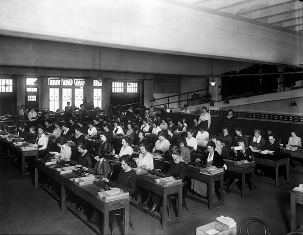
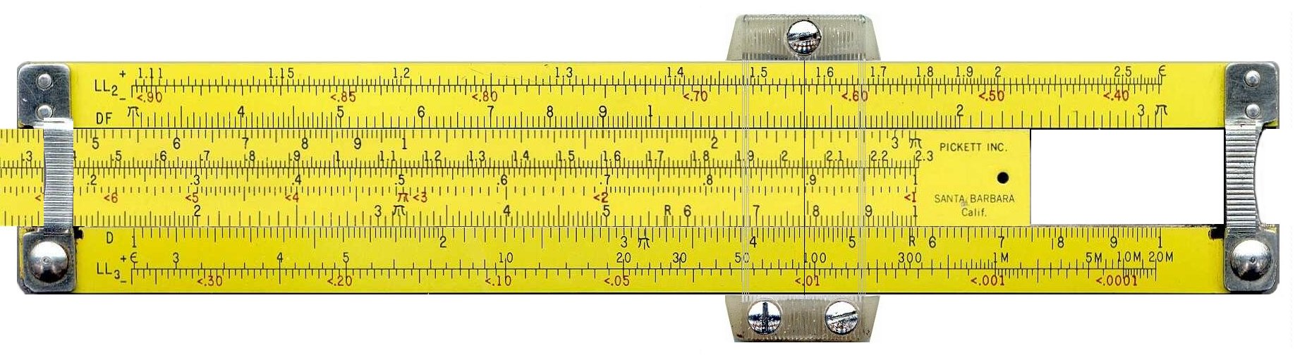
When Hestenes worked on conjugate bases in 1936, he was advised by a Harvard professor that it was too obvious for publication - CG doesn’t work on slide rules. - CG has little advantage over Gauss elimination for computation with calculators. - CG is not well suited for a room of human “computers” – too much data exchange.

Properties of the CG method

  • We need to store 3 vectors.

  • Since it generates A-orthogonal sequence p_1, \ldots, p_N, after n steps it should stop (i.e., p_{N+1} = 0.)

  • In practice it does not have this property in finite precision, thus after its invention in 1952 by Hestens and Stiefel it was labeled unstable.

  • In fact, it is a brilliant iterative method.

A-optimality

Energy functional can be written as

(Ax, x) - 2(f, x) = (A (x - x_*), (x - x_*)) - (Ax _*, x_*),

where A x_* = f. Up to a constant factor,

(A(x - x_*), (x -x_*)) = \Vert x - x_* \Vert^2_A

is the A-norm of the error.

Convergence

The CG method computes x_k that minimizes the energy functional over the Krylov subspace, i.e. x_k = p(A)f, where p is a polynomial of degree k+1, so

\Vert x_k - x_* \Vert_A = \inf\limits_{p} \Vert \left(p(A) - A^{-1}\right) f \Vert_A.

Using eigendecomposition of A we have

A = U \Lambda U^*, \quad g = U^* f, and

\Vert x - x_* \Vert^2_A = \displaystyle{\inf_p} \Vert \left(p(\Lambda) - \Lambda^{-1}\right) g \Vert_\Lambda^2 = \displaystyle{\inf_p} \displaystyle{\sum_{i=1}^n} \frac{(\lambda_i p(\lambda_i) - 1)^2 g^2_i}{\lambda_i} = \displaystyle{\inf_{q, q(0) = 1}} \displaystyle{\sum_{i=1}^n} \frac{q(\lambda_i)^2 g^2_i}{\lambda_i}

Selection of the optimal q depends on the eigenvalue distribution.

Absolute and relative error

We have

\Vert x - x_* \Vert^2_A \leq \sum_{i=1}^n \frac{g^2_i}{\lambda_i} \inf_{q, q(0)=1} \max_{j} q({\lambda_j})^2

The first term is just

\sum_{i=1}^n \frac{g^2_i}{\lambda_i} = (A^{-1} f, f) = \Vert x_* \Vert^2_A.

And we have relative error bound

\frac{\Vert x - x_* \Vert_A }{\Vert x_* \Vert_A} \leq \inf_{q, q(0)=1} \max_{j} |q({\lambda_j})|,

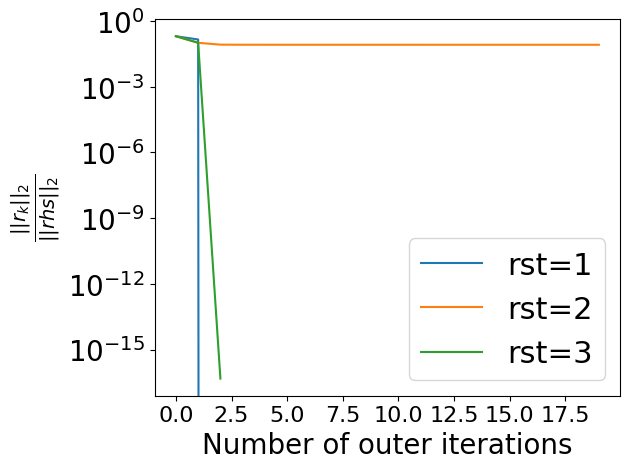
so if matrix has only 2 different eigenvalues, then there exists a polynomial of degree 2 such that q({\lambda_1}) =q({\lambda_2})=0, so in this case CG converges in 2 iterations.

  • If eigenvalues are clustered and there are l outliers, then after first \mathcal{O}(l) iterations CG will converge as if there are no outliers (and hence the effective condition number is smaller).

  • The intuition behind this fact is that after \mathcal{O}(l) iterations the polynomial has degree more than l and thus is able to zero l outliers.

Let us find another useful upper-bound estimate of convergence. Since

\inf_{q, q(0)=1} \max_{j} |q({\lambda_j})| \leq \inf_{q, q(0)=1} \max_{\lambda\in[\lambda_\min,\lambda_\max]} |q({\lambda})|

The last term is just the same as for the Chebyshev acceleration, thus the same upper convergence bound holds:

\frac{\Vert x_k - x_* \Vert_A }{\Vert x_* \Vert_A} \leq \gamma \left( \frac{\sqrt{\mathrm{cond}(A)}-1}{\sqrt{\mathrm{cond}(A)}+1}\right)^k.

Finite termination & clusters

  1. If A has only m different eigenvalues, CG converges in m iterations (proof in the blackboard).
  2. If A has m “clusters” of eigenvalues, CG converges cluster-by-cluster.

As a result, better convergence than Chebyshev acceleration, but slightly higher cost per iteration.

Summary

CG is the method of choice for symmetric positive definite systems:

  1. \mathcal{O}(n) memory
  2. Square root of condition number in the estimates
  3. Automatic ignoring of the outliers/clusters
  4. A-optimality property

Non-linear conjugate gradient method

Non-symmetric systems and the generalized minimal residual method (GMRES) (Y. Saad, M. Schultz, 1986)

Before we discussed symmetric positive definite systems. What happens if A is non-symmetric?

We can still orthogonalize the Krylov subspace using Arnoldi process, and get

A Q_j = Q_j H_j + h_{j,j-1}q_j e^{\top}_{j-1}.

Let us rewrite the latter expression as

A Q_j = Q_j H_j + h_{j,j-1}q_j e^{\top}_{j-1} = Q_{j+1} \widetilde H_j, \quad \widetilde H_j = \begin{bmatrix} h_{0,0} & h_{0,1} & \dots & h_{0,j-2} & h_{0,j-1} \\ h_{1,0} & h_{1,1} & \dots & h_{1,j-2} & h_{1,j-1} \\ 0& h_{2,2} & \dots & h_{2,j-2} & h_{2,j-1} \\ 0& 0 & \ddots & \vdots & \vdots \\ 0& 0 & & h_{j,j-1} & h_{j-1,j-1} \\ 0& 0 & \dots & 0 & h_{j,j-1}\end{bmatrix}

Then, if we need to minimize the residual over the Krylov subspace, we have

x_j = x_0 + Q_j c_j

and x_j has to be selected as

\Vert A x_j - f \Vert_2 = \Vert A Q_j c_j - r_0 \Vert_2 \rightarrow \min_{c_j}.

Using the Arnoldi recursion, we have

\Vert Q_{j+1} \widetilde H_j c_j - r_0 \Vert_2 \rightarrow \min_{c_j}.

Using the orthogonal invariance under multiplication by unitary matrix, we get

\Vert \widetilde H_j c_j - \gamma e_0 \Vert_2 \rightarrow \min_{c_j},

where we have used that Q^*_{j+1} r_0 = \gamma e_0, \gamma = \Vert r_0 \Vert

  • This is just a linear least squares with (j+1) equations and j unknowns.

  • The matrix is also upper Hessenberg, thus its QR factorization can be computed in a very cheap way.

  • This allows the computation of c_j. This method is called GMRES (generalized minimal residual)

Summary of the GMRES

  • Minimizes the residual directly
  • No normal equations
  • Memory grows with the number of iterations as \mathcal{O}(nj), so restarts typically implemented (just start GMRES from the new initial guess).
import scipy.sparse.linalg as la
from scipy.sparse import csc_matrix, csr_matrix
import numpy as np
import matplotlib.pyplot as plt
import time

%matplotlib inline
n = 150
ex = np.ones(n);
lp1 = sp.sparse.spdiags(np.vstack((ex,  -2*ex, ex)), [-1, 0, 1], n, n, 'csr'); 
e = sp.sparse.eye(n)
A = sp.sparse.kron(lp1, e) + sp.sparse.kron(e, lp1)
A = csr_matrix(A)
rhs = np.ones(n * n)

plt.figure(figsize=(10, 5))
f, (ax1, ax2) = plt.subplots(1, 2, figsize=(10, 5))
for restart in [5, 40, 200]:
    hist = []
    def callback(rk):
        hist.append(np.linalg.norm(rk) / np.linalg.norm(rhs))
    st = time.time()
    sol = la.gmres(A, rhs, x0=np.zeros(n*n), maxiter=200, restart=restart, callback=callback, tol=1e-16)
    current_time = time.time() - st
    ax1.semilogy(np.array(hist), label='rst={}'.format(restart))
    ax2.semilogy([current_time * i / len(hist) for i in range(len(hist))], np.array(hist), label='rst={}'.format(restart))
    

ax1.legend(loc='best')
ax2.legend(loc='best')
ax1.set_xlabel("Number of outer iterations", fontsize=20)
ax2.set_xlabel("Time, sec", fontsize=20)
ax1.set_ylabel(r"$\frac{||r_k||_2}{||rhs||_2}$", fontsize=20)
ax2.set_ylabel(r"$\frac{||r_k||_2}{||rhs||_2}$", fontsize=20)
plt.sca(ax1)
plt.yticks(fontsize=20)
plt.sca(ax2)
plt.yticks(fontsize=20)
f.tight_layout()
<Figure size 1000x500 with 0 Axes>

import scipy.sparse.linalg as la
import numpy as np
import matplotlib.pyplot as plt
%matplotlib inline

# Example from http://www.caam.rice.edu/~embree/39961.pdf

A = np.array([[1, 1, 1],
              [0, 1, 3],
              [0, 0, 1]]
            )
rhs = np.array([2, -4, 1])
x0 = np.zeros(3)

for restart in [1, 2, 3]:
    hist = []
    def callback(rk):
        hist.append(np.linalg.norm(rk)/np.linalg.norm(rhs))
    _ = la.gmres(A, rhs, x0=x0, maxiter=20, restart=restart, callback=callback)
    plt.semilogy(np.array(hist), label='rst={}'.format(restart))
plt.legend(fontsize=22)
plt.xlabel("Number of outer iterations", fontsize=20)
plt.ylabel(r"$\frac{||r_k||_2}{||rhs||_2}$", fontsize=20)
plt.xticks(fontsize=16)
plt.yticks(fontsize=20)
plt.tight_layout()

Next lecture

  • Iterative methods continued (BiCG, MINRES)
  • Preconditioners

Questions?

from IPython.core.display import HTML
def css_styling():
    styles = open("./styles/custom.css", "r").read()
    return HTML(styles)
css_styling()