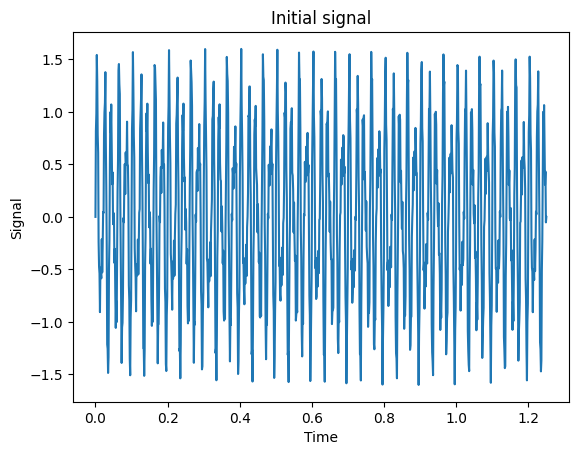
%matplotlib inlineimport matplotlib.pyplot as pltimport numpy as npN =1000dt =1.0/800.0x = np.linspace(0.0, N*dt, N)y = np.sin(50.0*2.0*np.pi*x) +0.5*np.sin(80.0*2.0*np.pi*x) +0.2*np.sin(300.0*2.0*np.pi*x)plt.plot(x, y)plt.xlabel('Time')plt.ylabel('Signal')plt.title('Initial signal')plt.savefig("signal.pdf")
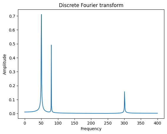
yf = np.fft.fft(y)xf = np.linspace(0.0, 1.0/(2.0*dt), N//2)plt.plot(xf, 2.0/N * np.abs(yf[0:N//2])) #Note: N/2 to N will give negative frequenciesplt.xlabel('Frequency')plt.ylabel('Amplitude')plt.title('Discrete Fourier transform')plt.savefig("fourier.pdf")
Быстрое преобразование Фурье
#FFT vs full matvecimport timeimport numpy as npimport scipy as spimport scipy.linalgn =10000F = sp.linalg.dft(n)x = np.random.randn(n)y_full = F.dot(x)full_mv_time =%timeit -q -o F.dot(x)print('Full matvec time =', full_mv_time.average)y_fft = np.fft.fft(x)fft_mv_time =%timeit -q -o np.fft.fft(x)print('FFT time =', fft_mv_time.average)print('Relative error =', (np.linalg.norm(y_full - y_fft)) / np.linalg.norm(y_full))
Full matvec time = 0.02279096011857142
FFT time = 6.669329407142856e-05
Relative error = 1.5259489891556028e-12